fast.ai 1.1.1: Data prep for “What’s that noise”

BLUF: Embarassing gory details of how I retrieved and prepared the data for my week 1 project with fast.ai. Here’s the main post where I talk about the context and results of this “work”.

Disclaimer: This is in no way a recommended or suggested method of doing this. This is just my hacky one-off homework workflow. In anything even remotely resembling a production setting I would’ve done all of these steps in a single script, or at least a single jupyter notebook. This hodgepodge is terrible. It’s non-reproducible, spread across about 4 different tools for a tiny hop of the data pipeline, and impossible to tweak, let alone “deploy”. Don’t be like me. Don’t do things this way. But, by jove, I still believe it’s better sometimes to spend 30min in Excel + bash to prove the sensibility of something than it is to overengineer from the start. Either way, it’s done, and I figure I may as well show the way I did it, for better or worse. Who knows, someone might learn something about awk along the way…

Overall, the dataset is pretty well structured. It consists of WAV files with some metadata, including a category and description for each sound. Sounds good — all I have to do is download all the sounds, sort them according to their assigned category, and convert the WAVs to a spectrograph. Then I can just follow the provided week 1 homework notebook, swapping out the input data for my image data.

The project homepage provides an interactive way to search for and listen to the sounds, which lets you discover gems such as “Half a dozen werewolves”, “Maniacal laughter (male and female)”, and “Execution being carried out with a block and sword” (which is distinct from “Execution being carried out with a block and large axe”). However, more usefully, there’s a downloadable index of the sounds (<- direct csv link!) available, so I started by downloading that.

Opening the data in Excel is always a good first move. Though eyeballing, the “sort and filter” tool, and some basic pivot tables, you can very quickly work out what you’re dealing with.

The metadata csv in Excel.

Looks pretty good. For a start, all the entries have a clear field for their WAV filename. I can tell from the “download” links on the project homepage that the URL prefix is constant, and they’re all just in a flat directory. So, at least it’ll be easy to programatically download them. I copied the base directory from the project homepage download links in the browser, and used the first sound file to do a test wget command in the terminal to ensure it worked:

base_url=http://bbcsfx.acropolis.org.uk/assets
wget base_url/07076051.wav

This revealed a few things. For a start, it Just Worked™! The BBC have been kind enough to make the files easily accessible, without having to deal with a structured API, weird HTTP authentication headers, and the like. So that’s one rabbit hole I didn’t need to go down. Before we go much further, I wanted to make sure I could turn these sound files into an image at all. A quick google brought up SoX, a command-line tool for sound processing, which includes a spectrograph command. Excellent. A quickbrew install sox later and I was off to the races. After a bit of man-page interpretation I found the correct command:

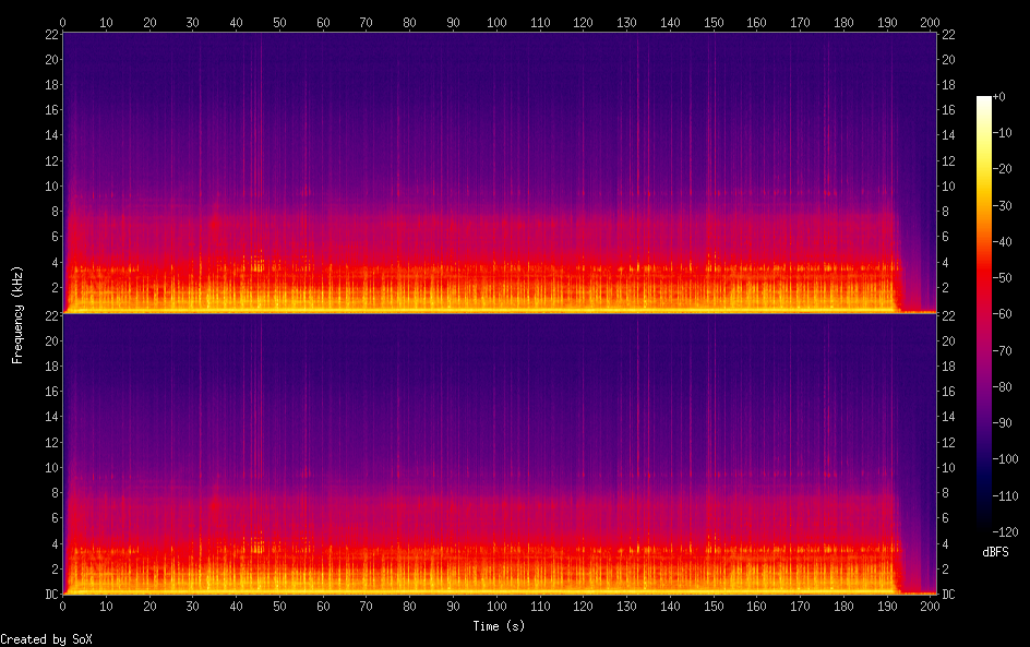
sox 07076051.wav -n spectrogram -o 07076051.wav.png

Which got me the lovely:

I humbly present “Two-stroke petrol engine driving small elevator, start, run, stop.”

Great! Now I’ve established I can download the sound files, and turn them into pictures. I already know how to do the rest. It looks like the project should be do-able! It’s worth testing these basic assumptions as early as possible.

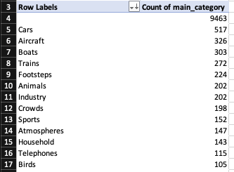
A more concerning discovery was that the file was much bigger than I expected. It was ~34MB for a 194 second (~3min) WAV. I did a quick sanity check: there are >16,000 files in this dataset; if this is even remotely the average size, the whole dataset would be (16000 * 34 / 1024) = 531GB! Even if the average is ~10x lower than that, I’d still be looking at >50GB of data for the whole dataset. With my slow internet connection and laptop SSD, this basically rules out downloading the whole lot. I’d have to pick just a few of the categories as a proof of concept. But which ones? I examined the categories to decide. A trivial Excel pivot table revealed another wrinkle:

I guess whoever categorised these sounds was really into their aviation.

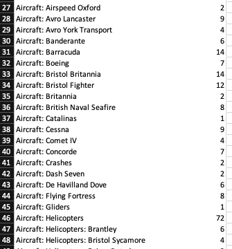
There are a lot of very specific categories with small numbers of samples. This is less than ideal; really we want as many samples per category as we can get, and anyway, I didn’t really want to teach a computer to tell the difference between an Avro Lancaster and an Avro York Transport (although it would be interesting to try later!). I grouped these into a higher-level category, i.e. just the word before the first colon. Easy enough with an Excel formula: =LEFT(H2, SEARCH(":",H2,1)-1). (For the sake of completeness: the cell that’s referencing isn’t actually the category cell; some of them were empty, and/or didn’t have a colon at all, so I introduced an interim cell which just appended a colon to the category,like so: =CONCAT(D4,":")). This gave me a fair few categories with at least 100 samples.

OK, now we’re getting somewhere.

So now what I wanted to do is download all the WAVs for the top few categories. I chose Cars, Aircraft, Boats and Trains, so the model can guess what kind of transport we’re using. I probably could’ve switched to Python at this stage, and debatably should’ve; but for whatever reason — mostly because I wanted to use SoX to do the conversion — my brain jumped to shell scripting. awk can split files by field, and wget can download files. So I thought it should be pretty straightforward to split the CSV into separate files based on the value of the “main_category” field, then use awk again on those files to extract the wav filename, then use wget to download the wav, then use SoX to turn the WAVs into pictures. Great. Off I went.

Of course, there were a few wrinkles with this, too. I had to export the file as a tab-separated file from Excel because there were commas in the comments field and awk isn’t quite smart enough to deal with that; I had to strip out the annoying line endings Excel exported the file with because they were producing really weird sed behaviour; I had to remove a forward slash in one of the category names; and I had to deal with the blank categories. All this took a lot of googling & hair-pulling to work out, but I got there in the end. I thought I was going to be able to use a command that looked like this:

awk -F\t '{print >> $9; close($9}'

And ended up with a frankencommand that looked like this:

cat ../BBCSoundEffects.tsv.txt | sed -e 's/^M//g' | awk -F\t '{gsub(/\//, "_", $9); ext=".tsv"; file=(length($9) > 2) ? ($9 ext) : "blank.tsv"; print >> file; close(file)}'

Anyway, now we ended up with a bunch of individual TSVs, one per category, containing the filenames of the WAVs in that category. Now it really is pretty straightforward. I made a little shell script to take some TSV names, and download the WAVs listed in that TSV into a directory named for that TSV’s category.

#!/bin/bash
bbc_dir="http://bbcsfx.acropolis.org.uk/assets/"
for f in $@
do
  dirname=${f%.*}
  mkdir -p $dirname
  echo "Created $dirname"
  cd $dirname
  for w in `awk -F\t '{print $1}' "../"$f`
    do
    wget -nv $bbc_dir$w
  done
  cd ..
done

In an effort to achieve “poor man’s parallel-but-throttled downloading” I kicked this script off 4 times:

../../scripts/download_wavs.sh Aircraft.tsv &
../../scripts/download_wavs.sh Boats.tsv &
../../scripts/download_wavs.sh Cars.tsv &
../../scripts/download_wavs.sh Trains.tsv &

And went to bed.

The next morning I was almost out of SSD space (600MB remaining!). There were almost 20GB of WAV files to deal with. I shunted them to an external HDD (I really should’ve thought of that before) and ran my SoX shell script:

#!/bin/bash
# Usage: create spectrographs for all wavs in the directory
shopt -s nullglob
for d in $@
do
  echo "looking at $d"
  for f in $d/*.wav
  do
    echo "Processing $f file"
    sox $f -n spectrogram -o $f.png
  done
done

I just ran this on all 4 directories (no need to parallelise as it’s perfectly quick). So, hurray! Now I had 4 directories with a couple hundred images each. Ready to start training!

…Well, almost. I had to put them into google drive so that my colab can see them. That’s a simple in-browser upload (although it was slow, because thanks Australian ADSL upload speeds). And with that, I was done.

Back to the article about the results.